Public-health data / Temporal modelling / Spatial analysis
Lassa Fever Forecasting
Testing forecasts across time. Making coverage visible.
A reproducible surveillance study for Liberia linking monthly data engineering, national forecasting, county model benchmarking, and GIS. Forward-in-time evaluation reveals where seasonal models add value and where sparse counts reward simple baselines.
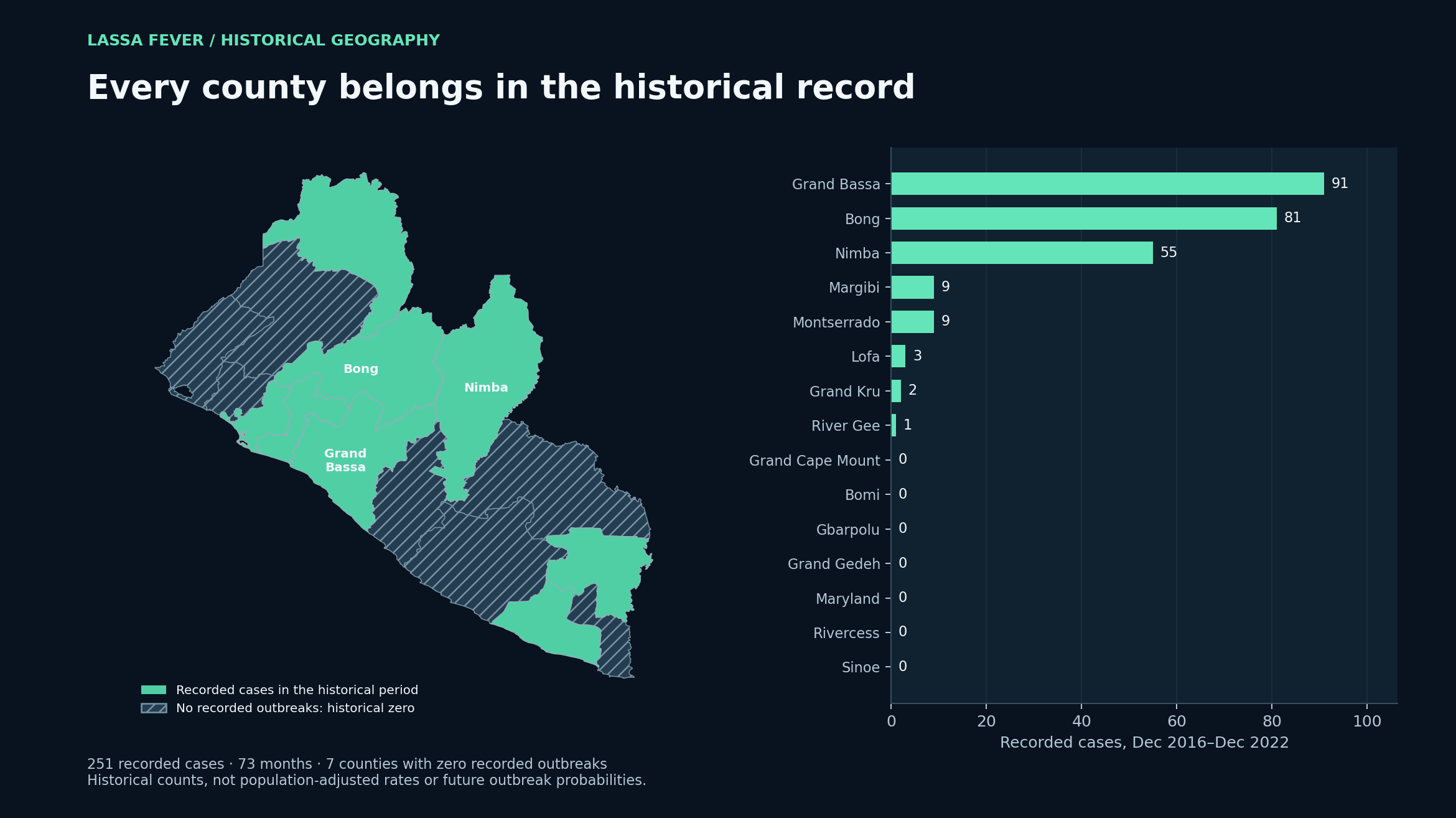
A complete view of the surveillance geography
01 / The question
When does forecasting add value to a sparse surveillance series?
Monthly surveillance counts raise two connected questions: how well can future national counts be forecast, and does a flexible county model improve on simple alternatives? The study evaluates both scales using only information available at each forecast origin. Historical zeros for counties with no recorded outbreaks remain part of the observed panel.
My contributionEngineered a complete 15-county monthly panel, implemented national and county forecasting pipelines, designed temporal backtests, and created maps and model-comparison figures.
02 / System walkthrough
From input to evidence.
The main stages of the implemented analytical workflow.
- 01
Build the observed panel
Reconcile county and national totals, validate dates and counts, and retain explicit historical zeros across all 15 counties.
- 02
Forecast forward in time
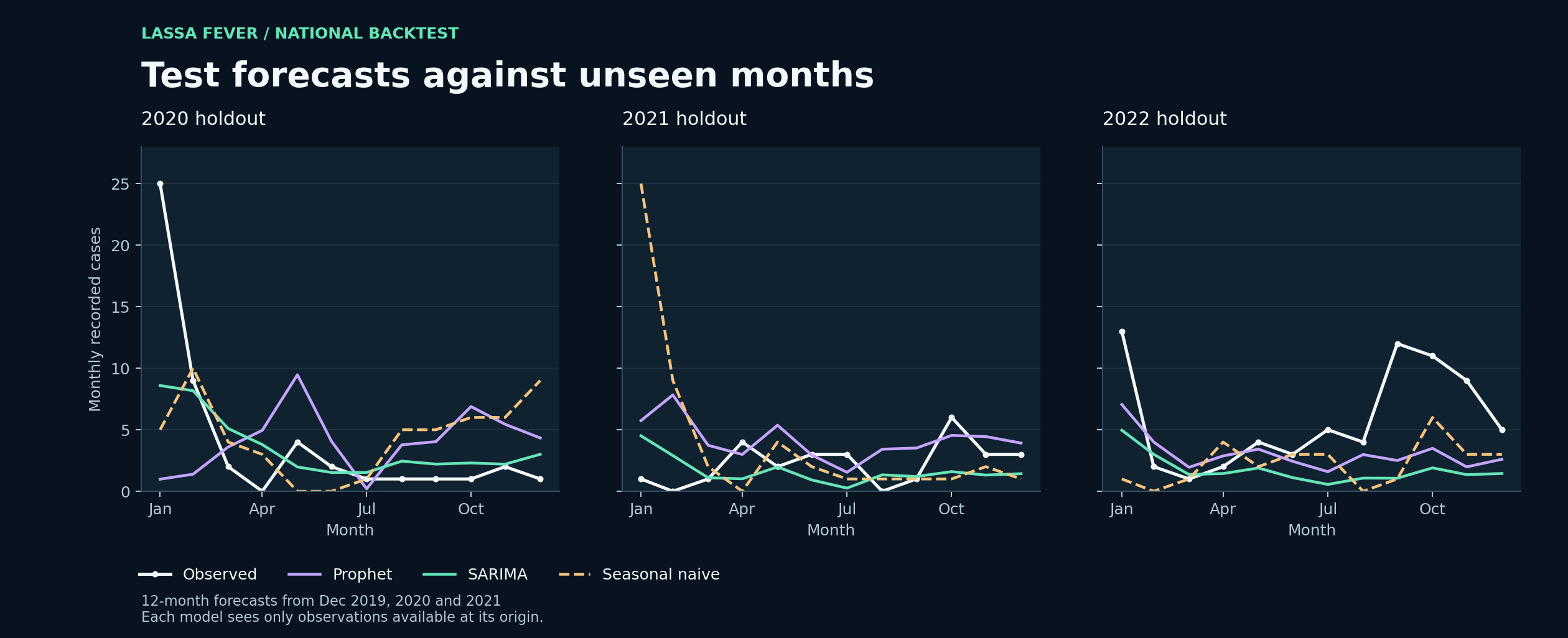
Train through December 2019, 2020, and 2021; forecast the following 12 months without using held-out outcomes.
- 03
Benchmark both scales
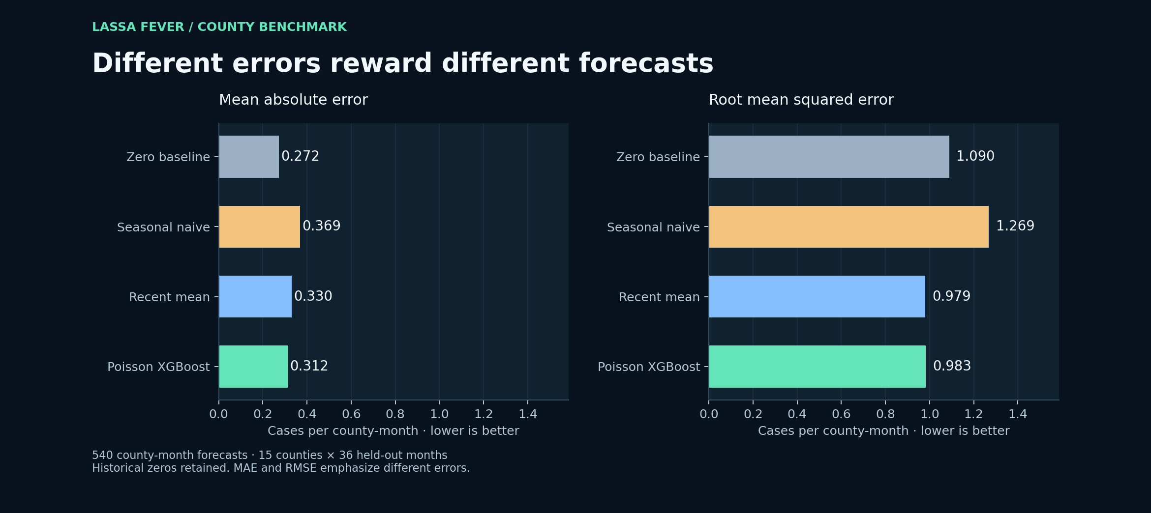
Compare SARIMA and Prophet with seasonal naive nationally; evaluate Poisson XGBoost against zero, seasonal-naive, and recent-mean county baselines.
- 04
Make results inspectable
Export metrics, convergence diagnostics, nonnegative projections, and responsive figures showing historical coverage and out-of-sample performance.
03 / Engineering decisions
Why the implementation matters.
Prevent target leakage
Lagged and rolling predictors use only prior months. Recursive forecasts feed earlier predictions into later steps; future outcomes are never filled with zeros.
Respect count support
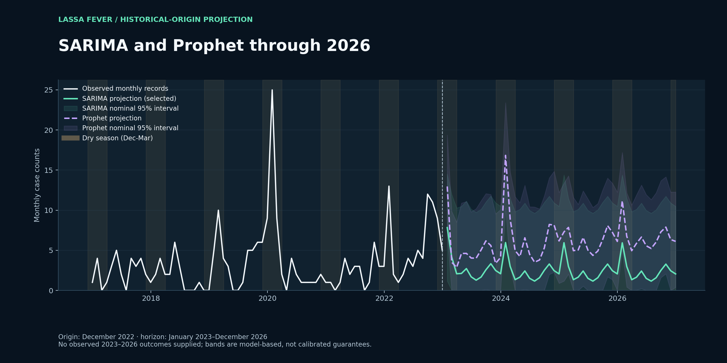
Poisson XGBoost models county counts. National point forecasts and interval endpoints are bounded below at zero.
Let baselines challenge complexity
Selection uses pooled MAE, while RMSE and year-by-year performance reveal different error tradeoffs. A simple county baseline can outperform a flexible model.
04 / Results & interpretation
What the experiment showed.
Rerun results from three 12-month rolling-origin backtests: 36 national months and 540 county–month predictions. Model selection uses pooled MAE.
National / SARIMA
3.04 MAELowest pooled national MAE: 30% below seasonal naive (4.36). Prophet scored 3.82; SARIMA did not win every year.
County / zero baseline
0.272 MAELowest pooled county MAE, compared with 0.312 for Poisson XGBoost. Sparse surveillance counts make baseline comparison essential.
County / error tradeoff
0.979 RMSERecent mean had the lowest county RMSE. Poisson XGBoost scored 0.983, versus 1.090 for the zero baseline.
Three forecast origins. One fair comparison.
Complexity earns its place through evaluation
SARIMA and Prophet through 2026
05 / Scope & limitations
Scope & limitations.
- Reported counts are not infection incidenceRecorded zeros are preserved as historical observations; they do not establish absence of infection or complete surveillance. Reporting completeness and changes in ascertainment require independent assessment.
- A short history and variable performanceThe series contains 73 months and only three annual forecast origins. SARIMA’s nominal 95% interval covered 32 of 36 held-out national months (88.9%); county intervals have not been calibrated.
- Historical-origin projectionsProjections through 2026 start from December 2022. Without subsequent observations, they are model scenarios rather than validated current forecasts. National and county projections are fitted separately and are not reconciled.
- Research scopeThis study evaluates forecasting and data handling, rather than demonstrating clinical utility, causal drivers, response effectiveness, or operational readiness.
06 / Next iteration
Where I would take it next.
The next technical priorities for this project.
Refresh and validate surveillance coverage
Add verified subsequent observations, reporting-completeness indicators, and denominators before interpreting geographic differences as risk.
Evaluate sparse-count alternatives
Compare hurdle and hierarchical count models with the same forward-in-time baselines; investigate how decisions change under MAE and RMSE.
Calibrate and reconcile uncertainty
Extend forecast origins, assess interval coverage by horizon, and evaluate coherent national–county forecasts.
07 / Code & reproducibility
Explore the implementation.
Explore the implementation, selected results, and technical documentation on GitHub.
- Corrected forecasting source with a synthetic-data example and pinned dependencies.
- Executed model metrics, convergence diagnostics, and a run manifest.
- Tests for lag construction, recursive prediction, input validation, and held-out target isolation.
Figures regenerated from the corrected pipeline and executed backtests. Only aggregate result summaries are published.